While we wait for the election results to be released later tonight, it would be useful to predict a priori what we would expect turnout to end up being. With an expectation established, based on past voting patterns in Wisconsin, it will be easier to assess how the unusual circumstances surrounding the primary may have affected turnout and the vote shares for candidates.
The exercise here is entirely empirical. There are too few data points—18 in all—to build an elaborate model. The main explanatory variable I will explore is the competitiveness of the presidential nomination fight.
A simple two-variable model of turnout
To start, I look at turnout in the presidential preference primary from 1948 to 2016, as a percentage of the voting-age population. Turnout is taken from the Wisconsin Elections Commission website, as is voting-age population, with the exception of 2012 and 2016, which I got from Michael McDonald’s United States Elections Project website.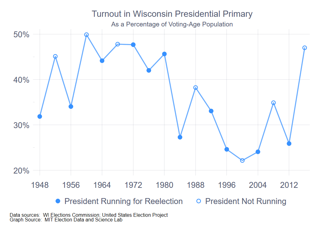 There are two notable patterns in the accompanying figure. (Click on any of the figures in this post to enbiggen.) First, there is a steep drop in turnout between the 1980 and 1984 primary. I’m not certain what caused this—it’s not due to the passage of the 26th Amendment to the U.S. Constitution, which gave 18-year-olds the right to vote, because that took effect with the 1972 election.
It has been suggested to me (thanks, Barry Burden) that prior to 1980, Wisconsin was typically early in the primary season, compared to other states, and thus a much more significant event in the hunt for the nomination. In any event, it is clear that 1984 and onward constituted a different turnout regime than the pre-1984 period. Whether the years prior to 1960 properly belongs to an even different period is an interesting question, but isn’t obviously relevant to the exercise of creating an expectation for turnout in 2020.
The exception to this simple periodization is 2016, where the turnout level of 47% was nearly twenty points higher than the average of the 1984 – 2012 period (29%). I will return to this point below.
The second pattern in the time series is the increase in turnout in years when the incumbent was not running for president, in other words, was precluded by the constitution from running for a third term. (Open-seat years are indicated with the open circles in the graph.) With the exception of 2000, the existence of a presidential open seat is associated with an increase in turnout in the primary, compared to the prior presidential election year. (And, one could possible even argue that Al Gore’s candidacy as Bill Clinton’s heir in 2000 meant that Gore was considered to be the de facto incumbent in the Democratic primary that year.)
The mechanism here is clear. With an incumbent president running for reelection, the in-party’s primary battle is typically subdued compared to the out-party’s. Absent another reason to come to the polls, the in-party’s partisans are likely to stay away to come degree. Conversely, in years where the incumbent cannot run for reelection, both parties tend to have hard-fought contests, drawing voters from both parties to the polls. 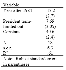 For starters, then, this suggests a simple regression model, where the dependent variable is turnout as a percentage of VAP and the independent variables are two dummy variables indicating (1) whether the year is 1984 or after and (2) whether the incumbent president is term-limited from running again. The results are in the accompanying table.
This allows for a simple prediction for 2020. With Trump not term-limited out, we would expect turnout in 2020 to be 40.6 – 13.2 = 27.4 percent of voting-age population. With VAP at 4,573,223, this works out to 1,253,063.
Adding competition
There is something unsatisfactory with models that rely solely on dummy variables, especially dummy variables demarking time periods, because they essentially say that nothing changes during the period in question, beyond random noise. Further examination of the graph above suggests there may be another dynamic at work, beyond whether the president is term-limited out, and that is the actual competitiveness of the races at hand.
For instance, in the post-war period, there were three elections in which both parties had hot nomination contests when the primary rolled around to Wisconsin—1980, which featured Kennedy and Carter duking it out on the Democratic side and Reagan and Bush locked in a tight race on the Republican side; 2008, with Clinton v. Obama and McCain v. Hckabee; and 2016, with Clinton v. Sanders and Cruz v. Trump and Kasich.
We can extend the previous regression model by adding the “effective number of candidates” measure to the mix. (See the end of this post to see a discussion of the effective number of candidates measure. In this case, I add the effective number of candidates in the two parties to create a unified variable. I do this to preserve degrees of freedom.)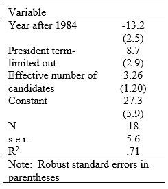 Doing so reveals the results in the accompanying table.
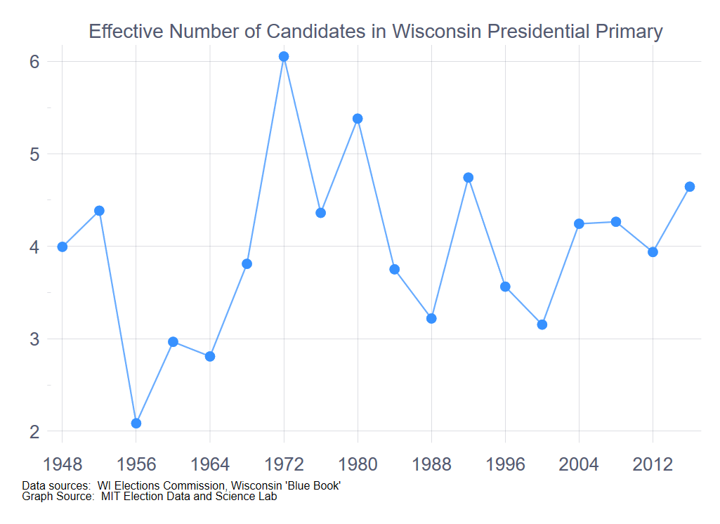
With the 2020 Republican primary uncontested and the Democratic primary down to two candidates, one of whom was already the presumptive nominee by primary day, the effective number of candidates for the 2020 primary was already among the lowest in the time series. In the best of cases, if Biden and Sanders tie, the effective number of candidates across the two parties would be precisely three—one for the Republicans plus two for the Democrats. As the following graph shows, the 2020 primary will likely be the least competitive Wisconsin presidential primary, considering the two parties together, since 1964.
To make a prediction from the regression model model, we have to estimate the results of the Democratic primary, while simplifying things by setting the effective number of Republican candidates to 1, ignoring scattering votes on the Republican side. The following table shows the range of estimates, varying the percentage of the vote for Biden from 30% to 70%, ignoring the vote for the other candidates.
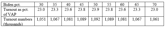
The high-end estimate, with a Biden-Sanders tie, is 23.9% of VAP, four points below what we predict without taking the non-competitive nature of the primary into account.
What about the 2016 outlier?
The one thing that makes me uneasy about these predictions is the 2016 primary turnout of 47%, the highest since 1980. Several commentators have suggested that 2016 had an especially high turnout because of the fiercely fought race for Wisconsin Supreme Court, between the liberal JoAnne Kloppenburg and the conservative Rebecca Bradley. (Wisconsin’s supreme court elections are non-partisan.) With the recent escalation of partisan rancor in the state, much of which has focused on Supreme Court decisions, the explanation for the turnout surge in 2016 could rest on the Supreme Court race, not the presidential primary.
 The fact that 2016 is truly an outlier is reinforced when we generate predicted values from the two regressions conducted above. The accompanying graph shows the actual time series, along with the two sets of predicted values from the regressions above. The 2016 values are 12 points greater than either regression would have predicted. This is similar in magnitude to the other outlier, 2000, where turnout was 13 points below what the model predicted.
On the issue of state supreme court races providing a turbo-boost to turnout in Wisconsin in general: if it did in 2016, it was the first time ever, at least in the post-war era. When I add variables intended to gauge the presence of contested supreme court races to the regression models above, nothing comes close to statistical significance. For instance, not all years have a supreme court race on the ballot. Adding a variable to account for supreme court races on the ballot along with the presidential primary adds nothing to the explanatory power of the two regression models, nor does adding a variable measuring how closely contested the supreme court race was.
The question, then, is whether 2016 was a true outlier, as was 2000, or whether 2016 ushered in a new partisan era. If it did, then we would expect turnout in 2020 to be about 15 points above what was predicted in the two regressions above. That is, we would expect turnout to be in the range of 1.8 and 1.9 million voters, depending on which regression model above is preferred. My political scientist training makes me skeptical about declaring new eras based on a single election, and so I would not expect turnout in 2020 to be nearly this high. Of course, with the confusion surrounding the primary, we may not know what the “new normal” is until 2024.
A conclusion (of sorts)
As of this writing, 1.1 million absentee ballots have been returned for counting. This guarantees that turnout based on absentee ballots alone with be in the ballpark of the predictions from the two regression models reviewed here. We still don’t know what total turnout is, because municipal clerks have hewed closely to the U.S. District Court order not to release any election results until Monday evening.
The Milwaukee City clerk has reported that about 20,000 voters cast ballots in person, anticipating that around 80,000 absentee ballots would eventually be returned. If these percentages hold for the whole state, then we’d anticipate for turnout to be around 1.4 million. Of course, Milwaukee’s in-person voting on Election Day was seriously hampered by the closing of over 90% of its Election Day precincts. I would expect that Wisconsin overall will see something less than 80% of its ballots cast by mail. If so, then turnout will be well above 1.4 million.
Either way, it seems reasonable to expect at this point that turnout will exceed what we should have expected, given the recent history of primaries in the state. Some may say that we should have expected much greater turnout, given the nature of the supreme court race also on the ballot, but one (or two) data points is a thin reed to hang such expectations on.
In any event, the fact that Wisconsin will likely see a much larger turnout for an uncompetitive presidential primary in the midst of a frightening pandemic says a lot about the persistence of the state’s voters and election workers, as it also says a lot about the likely level of turnout in November, when the obstacles to getting to the polls will (one hopes) not be so great.
Epilogue: The “Effective Number of Candidates” Measure
The “effective number of candidates” measure is analogous to the “effective number of parties” measure used in electoral studies to study the number of political parties in a system. Essentially, the effective number of candidates measure gauges how many candidates were on the ballot, weighting each candidate by the number of votes each received. If two candidates receive equal votes, the effective number of candidates is 2.0. If one candidate receives 90% and the other 10%, the effective number of candidates is 1.2. For the Democrats, the effective number of candidates was 1.5 when the incumbent Democrat was running for reelection, 1.8 when the seat was open, and 2.9 when a Republican was running for reelection. For the Republicans, the effective number of candidates was 1.3 when the incumbent Republican was running for reelection, 2.0 when the seat was open, and 2.5 when the Democrat was running for reelection.